Learning Outcomes
Upon completing this lesson, you will be able to:
- Articulate the formal definition of a function and identify if a relation is a function using algebraic and graphical methods.
- Utilize the Vertical Line Test as a definitive graphical tool for identifying functions.
- Define the concepts of domain and range and determine them for a given function by analyzing its algebraic structure.
- Classify a function as even, odd, or neither by performing an algebraic test for symmetry.
- Calculate the x- and y-intercepts of a function to identify key points on its graph.
Topics Covered
- Function Definition
- Domain and Range
- Symmetry
- Intercepts
I. Function Definition
A function is the fundamental object of study in calculus. Functions arise whenever one quantity depends on another. For example, the area of a circle depends on its radius, or the cost of mailing a package depends on its weight. To analyze these relationships, we must first have a precise definition of what constitutes a function.
A function $f$ is a rule that assigns to each element $x$ in a set $D$ exactly one element, called $f(x)$, in a set $R$.
The set $D$ is called the domain of the function. The range of $f$ is the set of all possible values of $f (x)$ as $x$ varies throughout the domain. A symbol that represents an arbitrary number in the domain of a function $f$ is called an independent variable. A symbol representing a number in the range of $f$ is called a dependent variable.
The most critical aspect of this definition is the uniqueness of the output. There can be only one corresponding output for any single, valid input. If a rule allows a single input to produce multiple outputs, it is merely a relation, not a function.
A. Formal Notation and Terminology
We use a standard notation: $f(x)$ to work with functions.
- $f$ is the name of the function. It acts as a label for the specific rule being applied.
- $x$ is the independent variable. It is a placeholder for any valid input value from the function’s domain.
- $f(x)$ is the dependent variable. It represents the output of the function, and its value is entirely dependent on the input value $x$. We often use the variable $y$ as a shorthand for $f(x)$, leading to the familiar equation form $y = f(x)$.
B. The Vertical Line Test
While the algebraic definition is precise, a graphical approach often provides more immediate insight. The Vertical Line Test is a simple and effective graphical method for determining whether a curve represents a function.
- Imagine a rigid vertical line sweeping across the graph from left to right.
- If this vertical line never intersects the curve at more than one point simultaneously, the graph represents a function.
- If, at any position, the vertical line intersects the curve more than once, the graph does not represent a function. This is because it visually demonstrates that a single x-value corresponds to multiple y-values.
Example 1
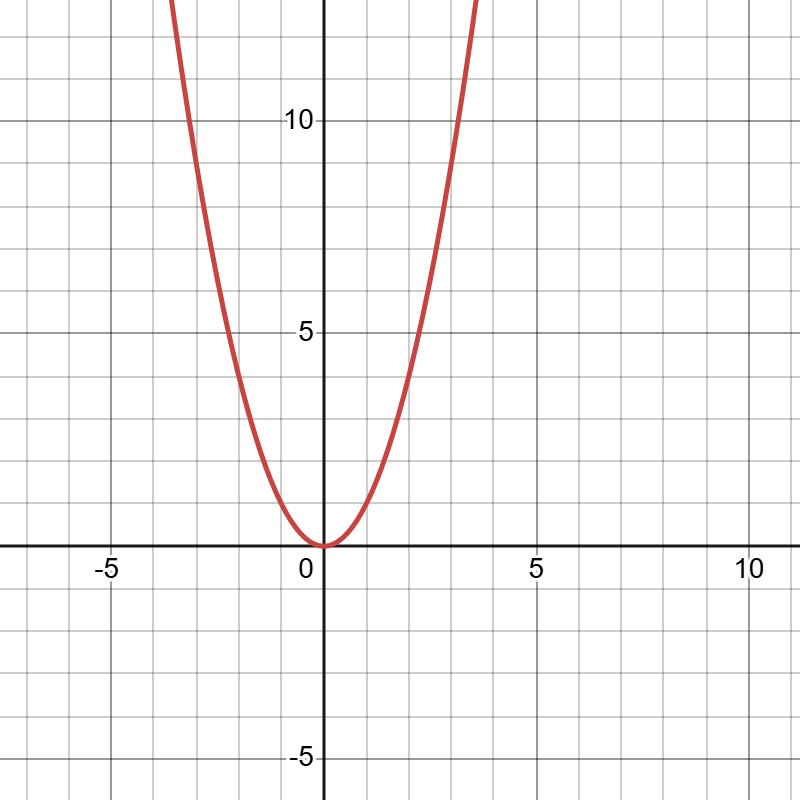
Consider the quadratic equation:
$$y = x²$$
This is a function because for any real number $x$ we choose as an input, there is only one possible output for $y$. If the input is $x = -1$, the output is unequivocally $y = (-1)² = 1$.
The graph of this equation is an upward-opening parabola, which will always pass the Vertical Line Test, as shown in Figure 2.
Example 2
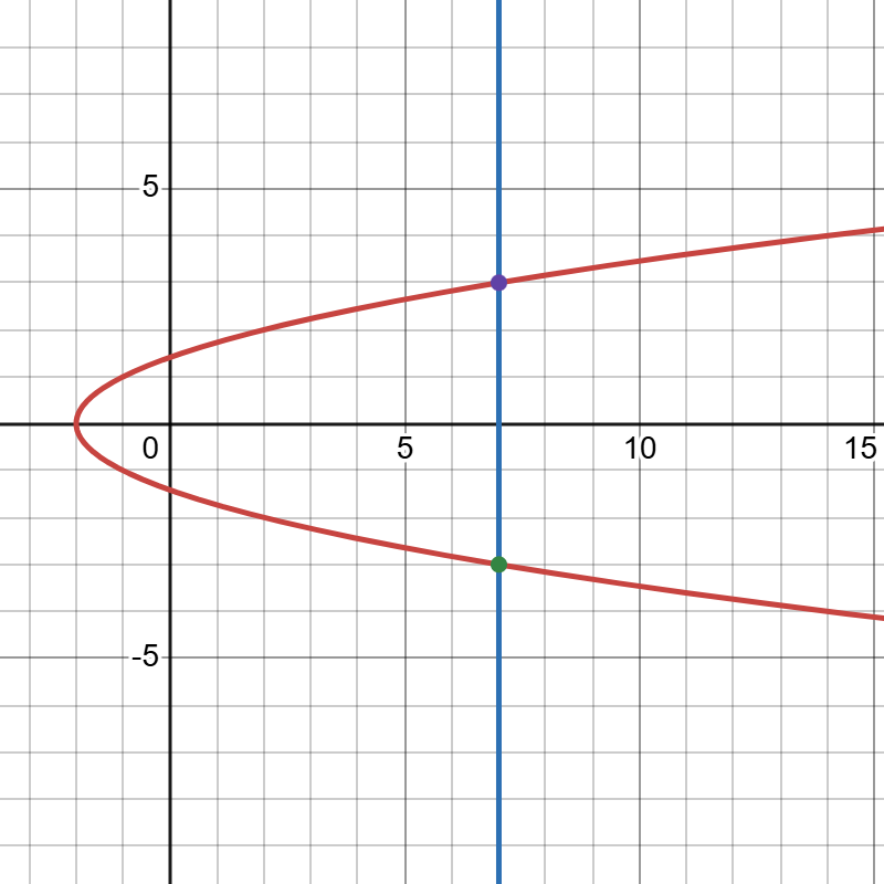
Consider the equation for a sideways parabola:
$$x = y² – 2$$
This relation is not a function of $x$. Let’s test the input $x = 7$. The equation becomes $7 = y² – 2$, which simplifies to $y² = 9$. This yields two distinct outputs: $y = 3$ and $y = -3$. The rule is violated since the single input x=7 leads to two outputs.
Its graph, shown in Figure 3, fails the Vertical Line Test.
C. Piecewise Functions
Sometimes, a single algebraic formula is insufficient to describe a complex relationship.
A piecewise-defined function is defined by multiple sub-functions, each applying to a different interval, or “piece,” of the domain.
The function is still a single, valid function, meaning each input from the entire domain maps to exactly one output. The key is first to determine which interval the input belongs to and then apply only the corresponding rule.
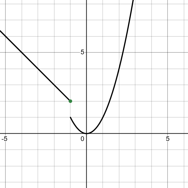
Example 3
Consider the function defined by:
$$f(x) = \begin{cases} 1-x & \text{if } x \le -1\\ x^2 & \text{if } x > -1\\ \end{cases}$$
We must first determine which rule to use based on the input to evaluate this function.
- To find $f(-2)$: Since $-2 <= -1$, we use the first rule: $f(-2) = 1 – (-2) = 3$.
- To find $f(-1)$: Since $-1 <= -1$, we use the first rule: $f(-1) = 1 – (-1) = 2$.
- To find $f(0)$: Since $0 > -1$, we use the second rule: $f(0) = (0)² = 0$.
The graph of this function (Figure 4) is constructed by drawing the line $y = 1-x$ for $x <= -1$ and the parabola $y = x²$ for $x > -1$.
II. Domain and Range
The domain and range are fundamental properties that define a function’s operational parameters. The domain specifies all the valid inputs the function can accept, while the range specifies all the possible outputs it can produce. Understanding these boundaries is the first step in analyzing any function’s behavior.
Note on Interval Notation: vs.
When describing sets of numbers, particularly for domains and ranges, we use interval notation. The symbols and [ are used to indicate whether the endpoint of the interval is included in the set.
Parentheses: – Exclusive
- What it means: The endpoint is not included in the set.
- Keywords: Think “open” or “exclusive”.
- Corresponds to: or .
Example: The interval represents all real numbers betw. and , not including or .
As an inequality:
Square Brackets: – Inclusive
- What it means: The endpoint is included in the set.
- Keywords: Think “closed” or “inclusive”.
- Corresponds to: or .
Example: The interval represents all real numbers betw. and 7, including and .
As an inequality:
A. The Domain: “What Inputs Are Allowed?”
The domain of a function is the complete set of all possible input values for which the function is mathematically defined and produces a real number output.
If the domain is not specified explicitly, the convention is that the domain is the set of all inputs for which the formula makes sense.
The standard strategy is to begin by assuming the domain is all real numbers , or , then identify and exclude any values that cause mathematical errors. Common restrictions arise from these primary rules:
- Division by Zero is Undefined: The denominator of any fraction cannot be zero. To find these restrictions, set the entire denominator equal to zero and solve for . The solutions are the values that must be excluded from the domain.
- Even Roots of Negative Numbers are Not Real: The expression inside a square root, fourth root, or any other even-indexed root (the radicand) must be non-negative (greater than or equal to zero). To find the domain, set the radicand greater than or equal to zero and solve the inequality.
It is important to note that odd-indexed roots (like a cube root, ) do not have this restriction and can accept any real number as input.
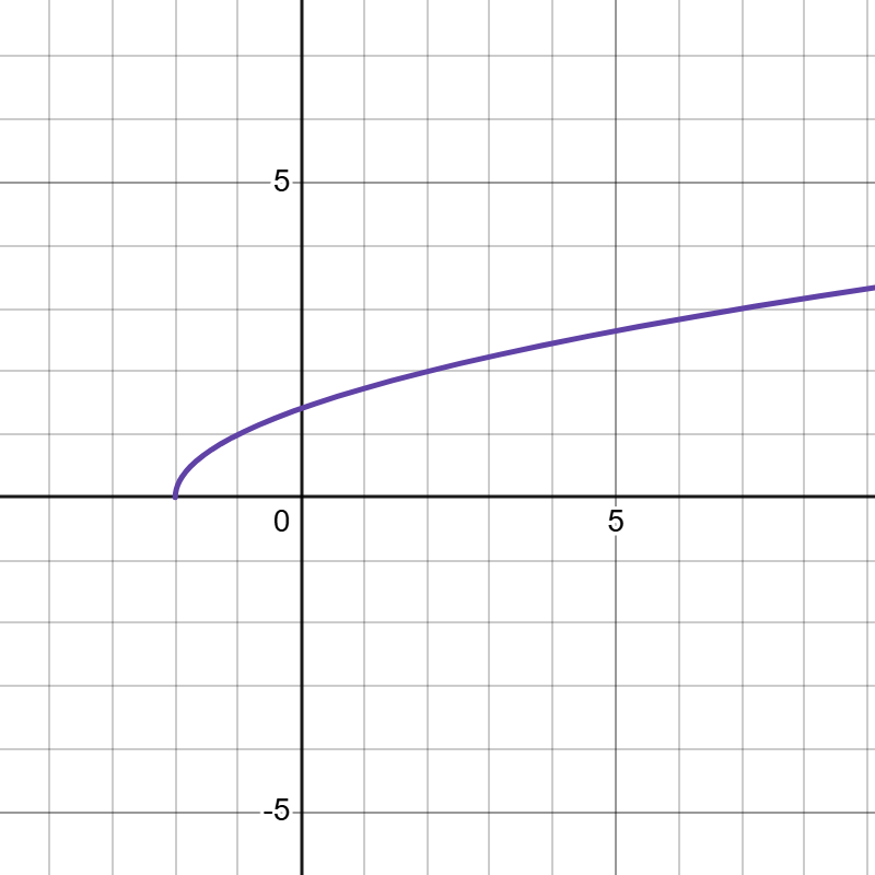
Example 4
Consider the Function as shown in Figure 5
The radicand must be non-negative: The domain is all real numbers greater than or equal to , written in interval notation as
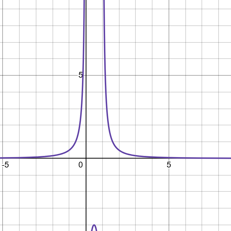
Example 5
Consider the Function as shown in Figure 6
we must ensure the denominator is not zero. We set the denominator to zero to find the excluded values: This implies . The domain is all real numbers except and . In interval notation, this is
B. The Range: “What Outputs Are Possible?”
The range of a function is the complete set of all possible output values that the function can produce from the inputs in its domain.
Determining the range can often be more complex than finding the domain and may require analyzing the function’s structure and behavior.
Here are some common strategies:
Analyze the Function’s Behavior and Known Properties:
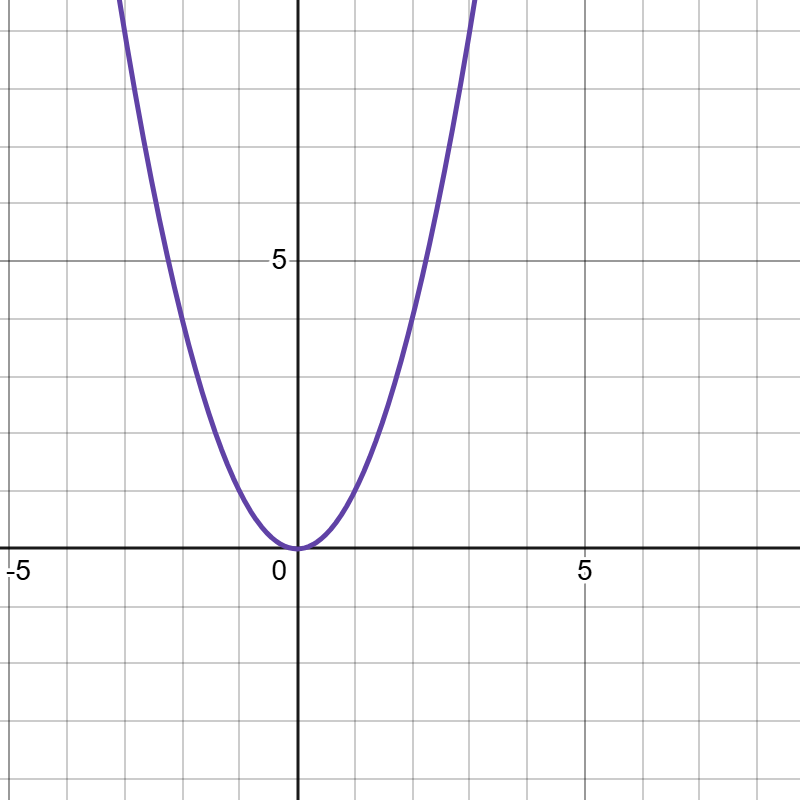
For a quadratic function like
As shown in Figure 7, we know that the term is always non-negative Therefore, the smallest possible value of is 0, and the range is
Consider the Parent Function and Transformations:
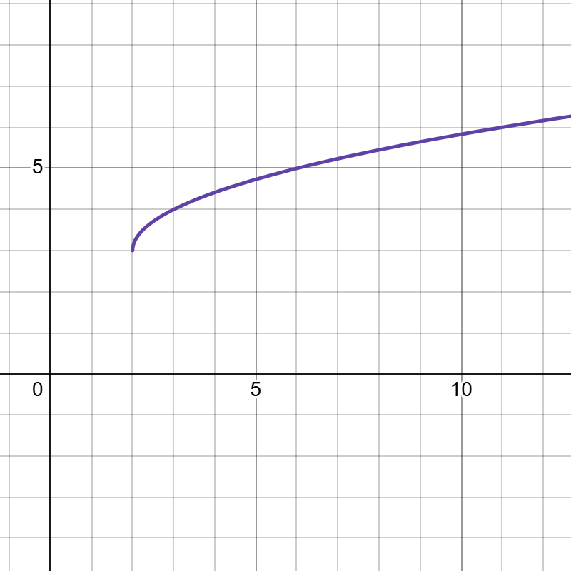
For a function like
We know the parent function, , has a range of . The transformation shifts the entire graph up by units as shown in Figure 8. Therefore, the new range is
Find the Inverse Function:
The range of a function is the same as the domain of its inverse function, . If the inverse can be found, determining its domain can reveal the original function’s range.
III. Symmetry
Symmetry describes the graphical balance and structure of a function. There are two primary types of symmetry: even and odd.
A. Even Functions (Y-Axis Symmetry):
A function is even if its graph is a mirror image across the -axis.
For every point on the graph, the point is also on the graph.
Algebraic Test: A function f is even if for all in the domain.
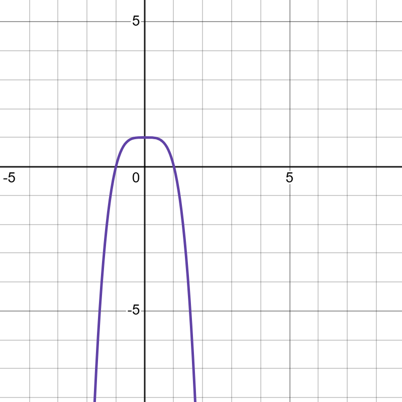
Example 6
Given as shown in Figure 9
Test: We evaluate :
Conclusion: Since , the function is even.
B. Odd Functions (Origin Symmetry):
A function is odd if its graph has rotational symmetry about the origin.
For every point on the graph, the point is also on the graph.
Algebraic Test: A function f is odd if for all in the domain.
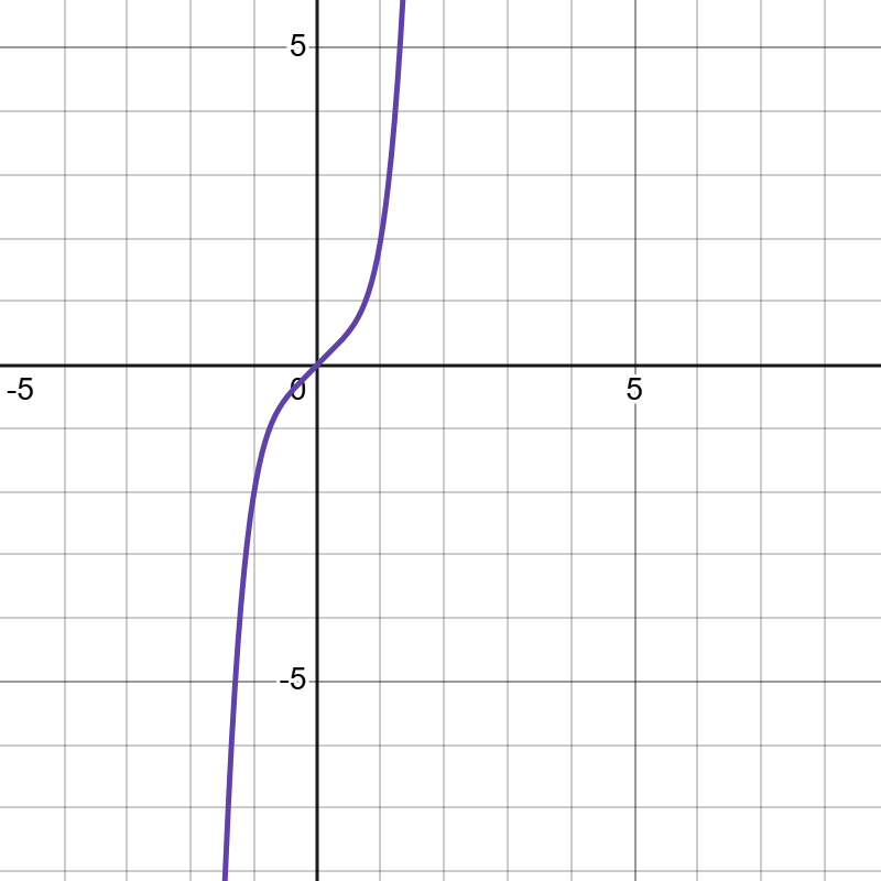
Example 7
Given as shown in Figure 10
Test: We evaluate :
Conclusion: Since , the function is odd.
C. Neither Even of Odd
If a function does not satisfy either of these tests, it is classified as neither even nor odd.
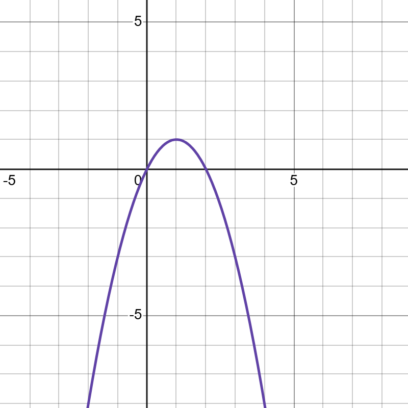
Example 8
Given as shown in Figure 11
Test: We evaluate :
Conclusion: The result is not equal to or , so the function is neither.
IV. Intercepts
Intercepts are the specific coordinates where a function’s graph crosses or touches the coordinate axes. These points are crucial as they provide concrete anchors for sketching and analyzing the graph.
Y-Intercept:
The point where the graph intersects the -axis.
At this point, the -coordinate is always . By the definition of a function, there can be at most one -intercept.
Calculation: To find the -intercept, set and solve for by computing .
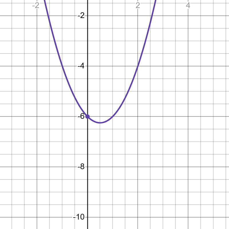
Example 9
Given as shown in Figure 12
Y-Intercept: We set :
The -intercept is at the point
X-Intercept:
The points where the graph intersects the -axis.
These points are also known as the roots or zeros of the function, because at these points, the output value is equal to .
Calculation: To find the -intercepts, set the function equal to zero and solve the equation for all real values of .
Example 10
Given as shown in Figure 13
X-Intercept: We set :
This quadratic equation can be factored:
The solutions are and .
The x-intercepts are at the points and .